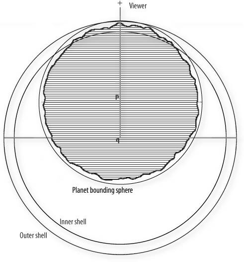
20.4. Atmospheric Effects

Atmospheric effects are vital for giving pictures of terrain their sense of scale. This section describes the atmospheric effects of aerial perspective and sky shading.

20.4.1. Aerial Perspective

The change in appearance of objects with distance is called "aerial perspective." Briefly, the Earth's atmosphere scatters blue light more than red light, so a distant object affords more opportunities for blue light to be scattered in the direction of the viewerso the object turns slightly blue, for the same reason that the sky is blue. Distant objects also tend to be darkertheir reflected light is more likely to be blocked by particles in the atmosphere.

The textbook method for calculating atmospheric scattering is described in the paper Display of The Earth Taking into Account Atmospheric Scattering, by T. Nishita, T. Shirai, K. Tadamura, E. Nakamae, in the SIGGRAPH '93 proceedings.

The standard way to calculate a distant object's change in color due to atmospheric effects is as follows. The change is split into "inscattering" and "extinction." Inscattering is the scattering of light into the line from object to eyethis is an addition in the light intensity. Extinction refers to the absorption of lightthis is a scaling of the light intensity by some factor. If L_o is the radiance of the distant object and L_s is the radiance of the ray at the viewer, then L_s = C_eL_o + C_i where C_e is the extinction factor, and C_i is the inscattered light.

In principle, this calculation should be done for each frequency of the light, but in practice it is acceptable to calculate the effect on only three wavelengthsthe standard red, green, and blue components. The extinction factor is calculated as C_e = exp(I · E · D) where I is the integral along the line from eye to object, E is the extinction ratio per unit length, and D is the density ratio. For a planet's atmosphere, the integrand is a spherically symmetric function.

The calculation of C_i has a similar formthe inscattering at each point along the object-eye line is integrated. The inscatter for a given point is a function of the angle between the sunlight and the line from the object to the eye, the density of the atmosphere, and the intensity of the sunlight reaching that point.

Leaving the mathematics at that point, we can see the extinction and inscattering contributions in Color Plate 37A, B, and C.

Previous work on real-time atmospherics have focused on height fields rather than full spherical planets; see, for instance, Rendering Outdoor Light Scattering in Real Time by Hoffman and Preetham. After several different attempts to find approximations of the required integrals for spherical atmospheres failed, we fell back to a simple but effective model that has little relation to the mathematics but is fast to compute and good enough to fool the eye. A diagram illustrating our approach and the arrangement of the relevant objects is shown in Figure 20.7.

This function we use is an approximation to 1.0 exp(I), where I is the integral through a distribution from the viewer (denoted by v) to the point x. This function takes the value 0 if v and x are coincident and rises to 1.0 if the line from v to x passes through high-valued regions of the distribution.

The function is made up of two components. The main termthe "atmospheric shell"follows the shape of the planet and provides a height-dependent effect, with distant objects more affected than close ones. The other term is a correction for the region near the viewer.

The planet is centered at the point p. The radius of the highest point on the terrain is found and establishes a bounding sphere for the planet. The position of the viewer, the point p, and the point q are collinear.

A function called the atmospheric shell is defined with center at the point q. Its value is a function of radius, taking the value 0 on the sphere marked "outer shell" and taking 1.0 on the "inner shell" sphere. Each shell's radius is fixed; the point q is chosen so that the outer shell is exactly tangent to the bounding sphere of the planet. The position of the point q is a function of viewer position. The radii of the inner and outer shell affect the distribution of the atmosphere; they are chosen by the planet artist. (They are exaggerated in Figure 20.7; in practice, the outer shell radius is usually not much more than the radius of the planet's bounding sphere.)

The value of the atmospheric shell function F₁ for a point x is

F₁ = (a ·|x - q|²) + b

where a and b are constants; they are chosen so the function takes the value 0 and 1.0 on the inner and outer shells, respectively. If r_o is the radius of the outer shell, and r_i is the radius of the inner shell, then

As described earlier, this function controls the amount by which the color is darkened and shifted to blue. A value of 0 causes no color changes; larger values cause a more pronounced color shift.

This function emulates the atmospheric color shift, decreasing with height and increasing with distance. Since the shell radii are larger than the planet radius, distant mountains are more affected by the color shift than are closer mountains. (It is possible to choose shell radii so that the shell function value does not monotonically decrease with distance from the viewer; this problem is usually because the radii are too small.)

But if the viewer approaches some terrain closely, then there should be no color shift; this function does not provide this effect, and so a second term was added to handle this case. The second term is a value proportional to exp(distance²):

F₂ = c · exp (|x - v|²) · d

The second term is subtracted from the first to provide the final value. The full fog calculation for a point x is as follows:

F_final = (a ·|x - q|²) + b - (c · exp (|x - v|²) · d

where q is the center of the atmospheric shell function, a and b are calculated from the inner and outer shell radii with the formula given described above, v is the viewer position, and c and d are constants determining the shape of the local visibility correction. As a final step, the computed value is clamped to the range [0,1].

This approximation is valid only for points within the planet bounding sphere. Points outside this sphere can be handled by being projected onto a sphere centered at the viewer whose radius is such that it intersects the planet bounding sphere at the horizon.

We tried several other atmospheric approximations without success. One common problem was that the value for a point on the terrain would change unrealistically as the viewer movedit did not monotonically increase or decrease as the viewer moved toward or away from the point; or the value did not monotonically decrease with terrain height. The atmospheric shell approximation described here is simply a fast function that displays the obvious characteristics a viewer expects, rather than an attempt to create a mathematically correct approximation.

The effect of the atmospherics is most clearly seen on the Snow planet, on which the atmosphere parameters have been pushed to an extreme to produce dense low-lying fog instead of subtle haze and color shift (see Color Plate 37E).

The transition from dense fog to clear air happens over a very short distance, so any problems with the atmospheric approximation function are more apparent. There are no artifacts or visible problems: The fog increases monotonically with height and with distance. There are no discontinuities, and the fog correctly follows the shape of the planet. Also, there are no temporal problems as the camera is moved.

The atmospheric approximation is not mathematically correct, but it is stable, fast, easy to implement, reasonably intuitive to work with, and good enough to fool the eye.

20.4.2. Sky Shading

The color of the sky is more complex and is shaded by means of a completely different technique. In RealWorldz, the approximation is made that sky color is a function of optical depth and the angle between sun and view direction. The function is expressed as a lookup table (texture map). Some images of the sky from the DragonRidges world are shown in Color Plate 37MT. The sky color texture for this planet is shown in Color Plate 37I, and its atmospheric density texture is shown in Color Plate 37J.

The sky color lookup table for DragonRidges produces a white sun, a blue sky, and a red sunset. The color of a pixel in a given direction, with a given optical depth is read from the sky color texture map. The y coordinate for the texture access is exp(O), where O is the optical depth. The resulting value is 1.0 for zero optical depth, and the function approaches zero as optical depth increases. The x coordinate for the texture access is the angle between the vector to the sun and the direction for the fragment in question, scaled to [0,1]. If the direction is exactly toward the sun, x is 0; if it is exactly away from the sun, x is 1.0.

The white vertical bar on the left-hand side of the DragonRidges sky color lookup table corresponds to low anglesdirections nearly pointing to the sun. This provides the sun glare. The top of the image fades to black, corresponding to the atmosphere fading out as it gets thinner. The right-hand side of the image corresponds to directions away from the sun; it is shades of blue that are darker for lower optical depth and brighter for higher optical depth. The reds and oranges in the lower left give the sunset effects for vectors that are somewhat in the sun's direction and travel through high-density atmosphere.

The alpha channel determines the blend between the cubemap with the stars and nebula and the atmosphere color. White means that the result is equal to the sky color; black means that the result is equal to the cubemap color. Grays indicate the different degrees of blend. This map is much the same for all the different atmospheres: white for the most part, with a smooth gradient establishing a transition to the star cubemap as optical depth decreases. A white bar runs the whole way up the left-hand side of the image so that the sun appears regardless of optical depth.

The calculation of optical depth is expensive, so the sky is rendered by means of a sphere centered on the viewer, tessellated into rings of fixed latitude, and rotated so that the axis is in line with the planet center. This arrangement is chosen specifically so that for a given latitude, the optical depth for any ray is the same. That way, the optical depth needs to be calculated once for each latitude.

For each vertex, exp(O) and direction are calculated. For the sky color texture map lookup in the fragment shader, two quantities are needed: the angle between the sun and the current direction for the x component, and exp(O) for the y component. It is sufficient to use the interpolated value provided by the vertex shader for the y component. Since finding the exact angle between two vectors with the acos function was deemed too slow, the x component is calculated as 0.25·|sd|², where s is the normalized sun direction vector and d is the normalized current direction. (For instance, if s and d are parallel, the result is zero; when the two are antiparallel, the length of their difference squared is 4.0, so the resulting x component is 1.0.)

This calculation is fast, but it yields a function that is quite dissimilar to the actual angle between two vectors. However, it is a monotonically increasing function of angle, so the inverse function can distort the texture map to compensate. For instance, the situation in which the sun and view direction are 18° apart corresponds to x = 18/180 = 0.1 in the above colormap. However, the x component calculation according to the new formula gives 0.09788. Therefore, the column of pixels at x = 0.1 is moved to x = 0.09788 to compensate. This resampling leads to a loss of detail in regions of low x; this loss is reduced when the corrected texture map is made twice the width of the source.

The body of the fragment shader is as follows:

// Vertex shader calculates s - d, and outputs deltaSD
float u = dot(deltaSD, deltaSD);

// expInvOpticalDepth = exp(-optical depth); this is the
// value calculated by the CPU described above
float v = expInvOpticalDepth;

// Sample the sky color texture map
vec4 atmosC = texture2D(skyColorTexturemap, vec2(u, v));

// Sample the star cubemap
vec4 starC = textureCube(starCubemap, worldDir);

// The blend between the sampled atmosphere color and the
// cubemap color is actually more sophisticated than a simple
// lerp: the star cubemap stores alpha as a measure of brightness,
// where 0.0 is very bright and 1.0 is dark. This code causes
// bright stars and moons to show through the atmosphere.

vec4 color = atmosC + (1.0 - (atmosC.a * starC.a)) * starC;

// colExtinction and colInscatter are due to atmospherics, and
// are calculated in the vertex shader

gl_FragColor = (color * colExtinction) + colInscatter;

The sky color texture maps could be procedurally generated, but since the lookup table is an image, it is natural to work on it with a paint program. Actions such as changing the color of the sky in some way (reddening, lightening, reducing contrast, etc.) can be done by application of that operation to the whole sky color texture map, which is much more intuitive than tweaking the parameters of a procedural model. Some of the sky color texture maps in RealWorldz were started by back-projection of reference photos of skies or sunsetscalculating the mapping from sky color texture map to screen, matching a sunset photo (for instance) and reversing the mapping to build the sky color texture map that gives the sunset image. Thus was defined the content of a small region of the texture map, which was then extended outward by being painted.

Painting the sky color texture map is very powerful, but it is not intuitive and has some pitfalls. For instance, finding the region of the texture map that controls the color of a particular piece of sky is not easy, so changing the color of one part of the sky without affecting anything else is difficult. One related problem is that the sky shader effectively distorts and smears the texture map to render the sky, so any sharp color changes in the texture cause very obvious lines in the sky. All such discontinuities have to be removed, but finding the problem area on the texture map is often the most time-consuming part of the process.

One example of an artistic effect that would be substantially more difficult to produce with a physically based atmosphere model is the halo around the sun on the Snow planet, as shown in Color Plate 37K. The rainbow around the sun was painted onto the texture; it is the subtle vertical rainbow visible on the left-hand side of the sky color texture map shown in Color Plate 37L.